source("patch-model.R")
fit <- calibrate_patches(n = 60000, seed = 2026, tolerance = 0.5)Exploring model parameters with tours
modelling
visualisation
R
Using tours to explore parameter relationships in infectious disease models.
Correlated parameters are fairly familiar territory when fitting infectious disease models. An increase in transmission can be balanced by a decrease in susceptibility, giving several parameter combinations that produce similar epidemics. This raises an identifiability question: which parameters, or combinations of parameters, can be estimated from the available observations? (Roosa and Chowell 2019)
A pairs plot is a useful way to explore these relationships. Plot each parameter against every other parameter, look for patterns, and try to explain what they mean for the model.
The relationship can also involve three or more parameters together. For example, increasing transmission in one population might be balanced by several different combinations of decreases in two others. In three dimensions, the fitted parameter sets could lie on a thin surface. Each panel of a pairs plot shows that surface from one direction, and can contain a surprisingly broad cloud of points.
This is where a tour is useful. A tour moves smoothly through different views of a dataset, allowing us to see its shape from different directions (Asimov 1985). It’s a fairly simple idea, and particularly helpful for exploring the parameter sets we get out of a model fit.
What is a tour?
A scatterplot gives us a view of a dataset along two axes. Usually, we choose two variables for those axes. A tour allows each axis to be a weighted combination of variables, then changes the weights smoothly to move between views.
With three parameters, this is similar to holding a cloud of points in front of you and turning it around. A flat surface looks broad when viewed face-on and narrow when viewed edge-on. Watching it turn helps us connect those two views and understand the shape.
The same idea works with more parameters. Each point might contain five, ten or twenty values, and we can still calculate two weighted combinations to position it on a screen. As the weights change, different aspects of the higher-dimensional structure come into view. We can follow individual points as groups separate, a cloud flattens, or an unusual observation moves away from the others.
Each view is a projection. You can think of it as a shadow of the full dataset cast onto a flat surface. Every point contributes to the display, and the movement comes from changing the viewing direction. In a model-fitting application, each point remains the same parameter set throughout.
Writing down a view
Suppose we have \(n\) parameter sets, each containing \(p\) parameters. Put them in an \(n \times p\) matrix \(X\), with one parameter set per row. For the following calculations, I’ll centre each column by subtracting its mean. This moves the cloud to the origin while retaining the original units and the differences between parameter sets.
A two-dimensional view is described by a \(p \times 2\) matrix
\[ A = \begin{bmatrix} | & |\\ \mathbf{a}_1 & \mathbf{a}_2\\ | & | \end{bmatrix}. \]
The columns of \(A\) give the weights for the horizontal and vertical axes. The displayed coordinates are then simply
\[ Y=XA. \]
For parameter set \(r\), its horizontal coordinate is \(\sum_{j=1}^p X_{rj}a_{j1}\), and its vertical coordinate is \(\sum_{j=1}^p X_{rj}a_{j2}\). A scatterplot of the first two parameters uses
\[ A = \begin{bmatrix} 1 & 0\\ 0 & 1\\ 0 & 0 \end{bmatrix} \]
when \(p=3\). Other choices allow all three parameters to contribute to the view.
The two columns are constrained to be perpendicular unit vectors:
\[ A^{\mathsf T}A=I_2. \]
This makes them an orthonormal basis for the viewing plane. The unit lengths give the two axes a common scale, and perpendicularity keeps them at right angles. As \(A\) changes, we can attribute changes in the displayed shape to the viewing direction. Projection discards the components perpendicular to the viewing plane, so distances can become smaller in a particular view.
In this notation, a tour is a continuous path \(A(s)\) through viewing planes, where \(s\) describes progress along the animation. Each frame displays \(Y(s)=XA(s)\).
Moving between views
A grand tour chooses a target plane at random and moves smoothly towards it. Once it arrives, it chooses another target. The interpolation maintains \(A(s)^{\mathsf T}A(s)=I_2\) throughout, giving us a continuous sequence of valid views.
In tourr, this movement uses geodesic interpolation: a shortest path between the planes under a distance defined by their principal angles (Buja et al. 2005; Wickham et al. 2011). We can calculate those angles from the current and target bases, \(A_0\) and \(A_1\), using a singular value decomposition:
\[ A_0^{\mathsf T}A_1 = U\,\operatorname{diag}(\cos\theta_1,\cos\theta_2)\,V^{\mathsf T}. \]
The \(\theta_j\) are the principal angles between the planes. The matrices \(B_0=A_0U\) and \(B_1=A_1V\) align their basis vectors into pairs, so each pair can be rotated through its corresponding angle.
For a non-zero angle, let \(\mathbf{b}_{0j}\) and \(\mathbf{b}_{1j}\) be the paired columns and define
\[ \mathbf{d}_j = \frac{\mathbf{b}_{1j}-\mathbf{b}_{0j}\cos\theta_j} {\sin\theta_j}. \]
The direction \(\mathbf{d}_j\) is perpendicular to \(\mathbf{b}_{0j}\). An intermediate direction is
\[ \mathbf{q}_j(s)= \mathbf{b}_{0j}\cos(s\theta_j) +\mathbf{d}_j\sin(s\theta_j), \qquad 0\leq s\leq 1. \]
At \(s=0\) we have the starting direction, and at \(s=1\) we have the target direction. A zero principal angle means that direction is shared by the planes, so it stays fixed. Collecting the \(\mathbf{q}_j(s)\) into a matrix gives an orthonormal basis at each step. Multiplying it by \(U^{\mathsf T}\) makes the path start with the original display axes; the endpoint spans the target plane.
The practical result is that nearby frames show nearby views. We can follow the same points as their projected positions change. The aps argument in the example below controls how quickly the tour travels along this path, and fps controls how many frames are displayed per second.
Choosing the path
There are several ways to choose the sequence of views:
- A grand tour moves between randomly selected projection planes, providing a general exploration of the dataset.
- A guided tour searches for views that score highly on a chosen measure, such as one that highlights separated groups (Cook et al. 1995).
- A manual tour lets the viewer control changes to the projection and investigate a particular relationship (Cook and Buja 1997).
The tourr package paper (Wickham et al. 2011) gives a fuller introduction to these ideas and their implementation in R. For the example here, I’ll use a grand tour generated by tourr, displayed in the page using detourr. The R code generates both the projection path and the interactive widget.
Three patches, three transmission rates
We have three patches, each with 100,000 people, and vaccination coverage of 20%, 45% and 70%. Vaccination happens before the simulation and gives perfect protection. Each patch starts with ten infectious people, the mean infectious period is five days, and 98% of potentially infectious contacts are within the same patch. The remaining 2% are split equally between the other two.
This is a deterministic SIR model. For patch \(i\),
\[ \begin{aligned} \lambda_i(t) &= \beta_i \sum_{j=1}^3 M_{ij}\frac{I_j(t)}{N_j},\\ \frac{\mathrm{d}S_i}{\mathrm{d}t} &= -\lambda_i(t)S_i(t),\\ \frac{\mathrm{d}I_i}{\mathrm{d}t} &= \lambda_i(t)S_i(t)-\gamma I_i(t),\\ \frac{\mathrm{d}R_i}{\mathrm{d}t} &= \gamma I_i(t). \end{aligned} \]
Here, \(\beta_i\) is the transmission rate associated with contacts made by susceptible people in patch \(i\), \(\gamma=1/5\) per day, and \(M\) is the mixing matrix described above. Vaccinated people start in \(R_i\), so \(S_i(0)=N_i(1-v_i)-10\), where \(v_i\) is the known vaccination coverage.
The three transmission rates are the unknowns. Everything else is fixed.
Suppose we observe the total number of new infections across all three patches over one week. Pooling the infections gives us one quantity to match when fitting the three transmission rates.
This allows the rates to compensate for each other. More infections in one patch can be balanced by fewer in the others. Vaccination coverage determines the initial susceptible population in each patch, and therefore how strongly each patch responds to a change in its transmission rate.
Fitting the weekly total
The model code simulates each proposed parameter set using a fourth-order Runge–Kutta solver with a quarter-day time step.
For this example, I generate a synthetic target using transmission rates \(\beta_i=0.26/(1-v_i)\). The target is the model’s expected weekly total, approximately 67.8 new infections, retained at full precision for the calibration.
I sample 60,000 parameter sets uniformly from a box with bounds \(0.22/(1-v_i)\) to \(0.30/(1-v_i)\) for each \(\beta_i\), then keep those whose predicted total is within half an infection of the target.
Those bounds put the reproduction numbers for isolated patches at approximately 1.1 to 1.5, before allowing for the small number already infectious. I’ve chosen this search region to give each patch a similar range of initial epidemic growth rates. A tight acceptance tolerance makes the resulting parameter relationships easier to see.
This leaves 3,120 accepted parameter sets. Together, they form a calibration ensemble: a collection of parameter combinations that reproduce the target within the chosen tolerance.1
First, the usual pairs plot:
pairs(fit$beta, pch = 16, cex = 0.3, col = "#26465335")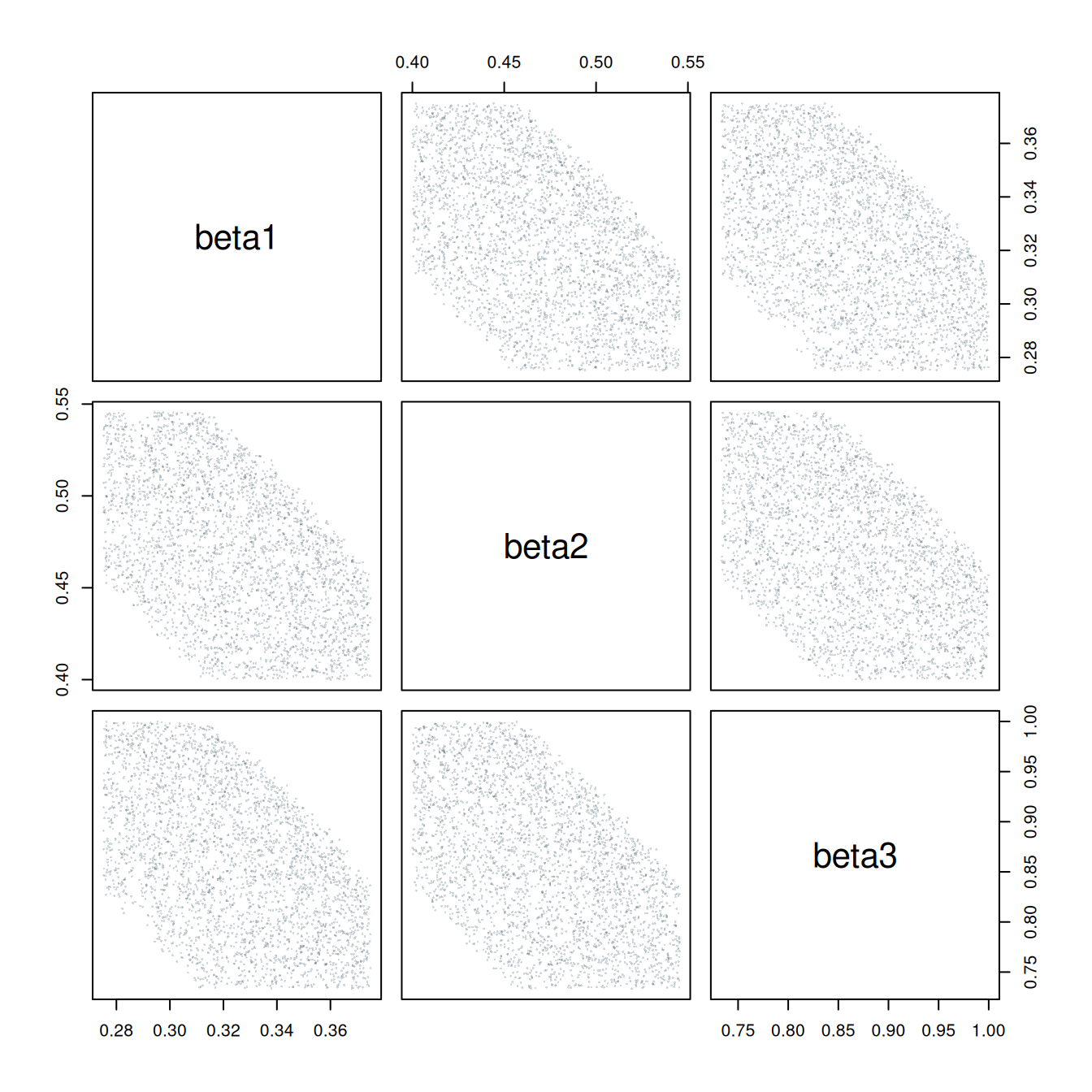
The pairwise correlations are all about \(-0.5\). Each panel shows the expected negative relationship, with a fairly broad range of values for one transmission rate at any given value of another. Let’s have a look at how these points fit together in three dimensions.
Enter the tour
We can pass the three transmission-rate columns directly to detourr. The tour_aes() mapping selects the parameters to project, grand_tour(d = 2) generates a path through two-dimensional views, and show_scatter() creates the interactive display.
I’ve fixed the random seed so the post shows the same path each time. The tour moves at half a radian per second, giving us time to follow the points between views.
Press play below, or drag the timeline to explore different views. Watch for the cloud turning almost edge-on. The labelled axes show how the three transmission rates contribute to the current projection.
library(tourr)
library(detourr)

set.seed(2026)

parameter_tour <- detour(
    as.data.frame(fit$beta),
    tour_aes(projection = beta1:beta3)
) |>
    tour_path(
        grand_tour(d = 2),
        aps = 0.5,
        fps = 30,
        max_bases = 20
    )

parameter_tour |>
    show_scatter(
        center = TRUE,
        axes = TRUE,
        paused = TRUE,
        alpha = 0.35,
        size = 2,
        height = 550
)As the cloud turns, it flattens into a narrow band and then spreads out again. The accepted parameter sets lie on a thin, slightly curved sheet. Seen edge-on, that sheet shows how tightly the three rates are related.
The input values are the original transmission rates, in units of per day. For display, detourr centres the cloud and applies one common scale factor to fit it in the widget. This preserves the relative distances between parameter sets. Each parameter retains its original scale relative to the others.
Exploring further in R
The code above can be run in an R session or included in a Quarto document. To explore parameter sets from another model, replace fit$beta with a data frame of draws or accepted parameter sets and select the relevant numeric columns in tour_aes().
For a tour in the R graphics window, tourr also provides:
library(tourr)

x <- fit$beta

animate(
    x,
    tour_path = grand_tour(d = 2),
    display = display_xy(),
    rescale = FALSE,
    sphere = FALSE
)
Here, rescale = FALSE and sphere = FALSE retain the relative parameter scales and covariance structure.
A useful feature of a tour is the movement itself. Following the same points between views makes it easier to understand how a broad cloud becomes a narrow band. When a view looks interesting, the projection coefficients tell us which combinations of parameters we’re looking at.
There are more directions to explore as the number of parameters grows, so it can take time to encounter a useful view. The same approach extends beyond three parameters: each display axis combines values across all the selected parameters.
What did the model actually tell us?
In this example, the constraint is the pooled weekly total:
\[ C(\boldsymbol{\beta}) = \sum_{i=1}^3 \{S_i(0)-S_i(7;\boldsymbol{\beta})\}. \]
Near a parameter set \(\boldsymbol{\beta}_0\), a first-order expansion gives
\[ C(\boldsymbol{\beta}_0+\Delta\boldsymbol{\beta}) \approx C(\boldsymbol{\beta}_0) +\nabla C(\boldsymbol{\beta}_0)^{\mathsf T}\Delta\boldsymbol{\beta}. \]
Where the gradient is non-zero, changes that preserve the total approximately satisfy
\[ \nabla C(\boldsymbol{\beta}_0)^{\mathsf T}\Delta\boldsymbol{\beta}=0. \]
This describes a plane of local trade-offs, perpendicular to the gradient. There are two directions along that plane in which the three rates can compensate for each other. The tight acceptance tolerance restricts movement in the perpendicular direction, giving the sheet its small thickness. Its curvature comes from the nonlinear relationship between the transmission rates and the epidemic dynamics.
The projection formula also explains how the tour reveals this relationship. If \(\Sigma\) is the covariance matrix of the accepted parameter sets, the covariance in a view with basis \(A\) is
\[ \operatorname{Cov}(XA)=A^{\mathsf T}\Sigma A. \]
In particular, the variance along a unit direction \(\mathbf{a}\) is \(\mathbf{a}^{\mathsf T}\Sigma\mathbf{a}\). A view with one axis close to the sheet’s normal direction therefore has little spread along that axis. The other axis can still show substantial variation along the sheet, producing the narrow band in the animation.
Each panel of a pairs plot uses two original coordinate directions. A tour explores combinations of those directions, including views that bring this small joint variation into the display. For a curved surface, the normal direction varies across the cloud; the edge-on band retains some curvature and width.
The pooled observation is central to this example. Patch-specific observations or a longer time series could provide additional constraints on the rates. Comparing those fits with this one would let us investigate how the parameter relationships change as more information becomes available.
Weak mixing and unequal vaccination coverage describe the setting. Their individual effects on the shape of the parameter cloud would need to be investigated by varying them.
For other models, the parameter scales also deserve some thought. Keeping the original units works well here because all three parameters are transmission rates. Parameters measured in very different units may benefit from scaling, with the choice made explicit so we can interpret the resulting views.
Another way to look at a model fit
The three-dimensional relationship in this example is easy to explain once we’ve seen the sheet. Each pairs-plot panel shows a broad range of possibilities because the third parameter can vary too. Watching the points rotate brings those views together.
This is what I find useful about tours. They give us a practical way to explore relationships involving several parameters, using the parameter sets we already have. A few lines of R are enough to start looking.
If you’ve fitted a model with several parameters, try putting the results through a tour. I’d be interested to hear what you find.
References
Asimov, Daniel. 1985. “The Grand Tour: A Tool for Viewing Multidimensional Data.” SIAM Journal on Scientific and Statistical Computing 6 (1): 128–43. https://doi.org/10.1137/0906011.
Buja, Andreas, Dianne Cook, Daniel Asimov, and Catherine Hurley. 2005. “Computational Methods for High-Dimensional Rotations in Data Visualization.” In Data Mining and Data Visualization. Handbook of Statistics. Elsevier. https://doi.org/10.1016/S0169-7161(04)24014-7.
Cook, Dianne, and Andreas Buja. 1997. “Manual Controls for High-Dimensional Data Projections.” Journal of Computational and Graphical Statistics 6 (4): 464–80. https://doi.org/10.1080/10618600.1997.10474754.
Cook, Dianne, Andreas Buja, Javier Cabrera, and Catherine Hurley. 1995. “Grand Tour and Projection Pursuit.” Journal of Computational and Graphical Statistics 4 (3): 155–72. https://doi.org/10.1080/10618600.1995.10474674.
Roosa, Kimberlyn, and Gerardo Chowell. 2019. “Assessing Parameter Identifiability in Compartmental Dynamic Models Using a Computational Approach: Application to Infectious Disease Transmission Models.” Theoretical Biology and Medical Modelling 16 (1): 1. https://doi.org/10.1186/s12976-018-0097-6.
Wickham, Hadley, Dianne Cook, Heike Hofmann, and Andreas Buja. 2011. “tourr: An R Package for Exploring Multivariate Data with Projections.” Journal of Statistical Software 40 (2): 1–18. https://doi.org/10.18637/jss.v040.i02.
Footnotes
The ensemble depends on the sampling box and acceptance tolerance. A posterior analysis would additionally require a probabilistic observation model and priors.↩︎